Post
Time series anomaly detection using PCA
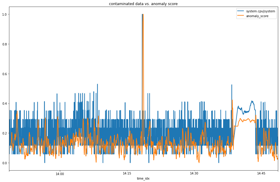
contaminated raw data vs anomaly score
Here is a little recipe for using good old PCA to do some fast and efficient time series anomaly detection.
The high level idea here is to:
- “featurize” the time series data into a traditional feature vector based formulation over recent data.
- fit a PCA model on some “mostly” normal data.
- when new data arrives if the PCA model is not able to do a good enough job at representing that data then that could be a sign of some anomalous observations.
- use some min/max normalisation tricks on the training data to get a nice “anomaly score” on a 0-100 scale.
Note: You can run and play with this colab notebook if you’d rather just look at the code (github, colab).
Raw Data
Let’s begin by getting some raw data to work with. Here i will use public data from a demo server at Netdata Cloud where i work. You can see this data on the Netdata dashboard here or via its api here (which is what we will be using - albeit via our netdata_pandas package that manages all that).
# inputs
host = 'london.my-netdata.io'  # pull from 'london' netdata demo host
after = -3600  # last 60 minutes
before = 0  # starting from now
dims = ['system.cpu|system']  # lets just look at syatem cpu data

# params
n_train = 3000  # use the last 50 minutes of data to train on
diffs_n = 1  # take differences
lags_n = 3  # include 3 lags in the feature vector
smooth_n = 3  # smooth the latest values to be included in the feature vector

# get raw data
df = get_data(
    hosts=[host],
    charts=list(set([d.split('|')[0] for d in dims])),
    after=after,
    before=before,
    index_as_datetime=True
)
df = df[dims]

# look at raw data
print(df.shape)
display(df.head())
This gives us our raw data from the last 60 minutes that we will be using.
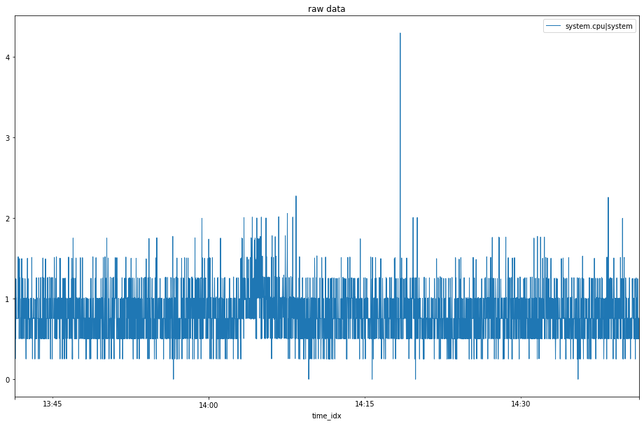
raw data
Add some anomalies
To make things easy on ourselves we will take a little snippet of time towards the end of our raw data and mess it up by first shuffling it and then smoothing it so that it’s clearly anomalous.
# create anomalous data
anomalous_len = int((len(df) - n_train) / 2)  # we pick half of our anomalous window to mess up
df_anomalous = df.tail(anomalous_len + anomalous_len)  # get the tail end of our raw data
df_anomalous = df_anomalous.head(anomalous_len)  # take the top part of it we want to mess with
df_anomalous[dims] = df_anomalous.sample(frac=1).values  # scramble the data
df_anomalous = df_anomalous.rolling(60).mean()*2  # apply a 60 seconds rolling avg to smooth it so that it looks much different

# append train data and anomalous data as 'contaminated' data
df_contaminated = df_train.append(df_anomalous).append(df.tail(anomalous_len)).interpolate(method='linear')
df_contaminated.plot(title='contaminated data', figsize=(16,10), lw=1)
Now we have data that look’s like below.
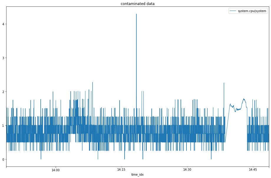
data with anomalous period added it
Preprocessing
I have not mentioned it much but a key part of this “recipe” is in how we preprocess or featurize our raw time series data. We are keeping it simple here by ‘fattening’ our time series data at each timestep into a differenced, smoothed and lagged feature vector (which we also take absolute values of). This is typical basic feature preprocessing you might to when you want to convert your time series data into a more traditional ML formulation of observations of X’s and y’s.
I won’t talk about this much but here is a great blog post (all his stuff is great) that covers things in more detail.
def preprocess_df(df, lags_n, diffs_n, smooth_n, diffs_abs=False, abs_features=True):
    """Given a pandas dataframe preprocess it to take differences, add smoothing, and lags as specified.
    """
    if diffs_n >= 1:
        # take differences
        df = df.diff(diffs_n).dropna()
        # abs diffs if defined
        if diffs_abs == True:
            df = abs(df)
    if smooth_n >= 2:
        # apply a rolling average to smooth out the data a bit
        df = df.rolling(smooth_n).mean().dropna()
    if lags_n >= 1:
        # for each dimension add a new columns for each of lags_n lags of the differenced and smoothed values for that dimension
        df_columns_new = [f'{col}_lag{n}' for n in range(lags_n+1) for col in df.columns]
        df = pd.concat([df.shift(n) for n in range(lags_n + 1)], axis=1).dropna()
        df.columns = df_columns_new
    # sort columns to have lagged values next to each other for clarity when looking at the feature vectors
    df = df.reindex(sorted(df.columns), axis=1)

    # abs all features if specified
    if abs_features == True:
        df = abs(df)

    return df

# preprocess or 'featurize' the training data
train_data = preprocess_df(df_train, lags_n, diffs_n, smooth_n)

# preprocess or 'featurize' the anomalous data
anomalous_data = preprocess_df(df_anomalous, lags_n, diffs_n, smooth_n)

# preprocess or 'featurize' the contaminated data
contaminated_data = preprocess_df(df_contaminated, lags_n, diffs_n, smooth_n)
PCA FTW!
Now lets fit our PCA model on our training data and then use it to derive some anomaly scores for our anomalous data.
First we need to define exactly how we are going to use the PCA model to derive our anomaly scores.
def anomaly_scores(pca, X):
    """Given a fitted pca model and some X feature vectors, compute an anomaly score as the sum of weighted euclidean distance between each sample to the
    hyperplane constructed by the selected eigenvectors.
    """
    return np.sum(cdist(X, pca.components_) / pca.explained_variance_ratio_, axis=1).ravel()
The function above takes in a fitted PCA and X vector of feature vectors and then computes a weighted distance measure between the features and the principle components. In a hand wavy sense the idea here is to measure the reconstruction error between the features X and our learned lower level representation of them that is implied via the fitted PCA mode (more details and references can be found in the awesome PyOD docs - p.s. if you can you should just use PyOD as it has lots of different models implemented).
Now all we have to do is train or model, score our contaminated data and then apply our last little trick of min/max normalizing the raw anomaly scores based on the scores observed within the training data.
# build PCA model
pca = PCA(n_components=2)

# scale based on training data
scaler = StandardScaler()
scaler.fit(train_data)

# fit model
pca.fit(scaler.transform(train_data))

# get anomaly scores for training data
train_scores = anomaly_scores(pca, scaler.transform(train_data))
df_train_scores = pd.DataFrame(train_scores, columns=['anomaly_score'], index=train_data.index)
df_train_scores_min = df_train_scores.min()
df_train_scores_max = df_train_scores.max()

# normalize anomaly scores on based training data
df_train_scores = ( df_train_scores - df_train_scores_min ) / ( df_train_scores_max - df_train_scores_min )

# score all contaminated data
contaminated_scores = anomaly_scores(pca, scaler.transform(contaminated_data))
df_contaminated_scores = pd.DataFrame(contaminated_scores, columns=['anomaly_score'], index=contaminated_data.index)

# normalize based on train data scores
df_contaminated_scores = ( df_contaminated_scores - df_train_scores_min ) / ( df_train_scores_max - df_train_scores_min )
Now we can see we have our lovely normalized anomaly scores as below where we can see a clear elevation in the anomaly score during our anomalous window.
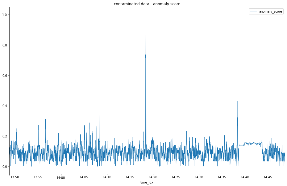
normalized anomaly scores
As one last little bit of post processing we can apply a rolling average to our normalized anomaly scores to try and make our anomalous window stand out a little more.
df_contaminated_scores_smoothed.plot(title='contaminated data - smoothed anomaly score', figsize=(16,10), lw=1)
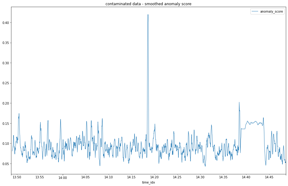
smoothed normalized anomaly scores
And there you have it, a fairly simple recipe with a bit of sensible feature engineering, good old reliable PCA, little normalization trick and you have a fairly robust, efficient and easy to implement anomaly detection playbook.
Comments